A reasonable probability is the only certainty. - E.W. Howe The best way to describe the term "Probability" is that its a combination of very interesting concepts with 500 things to keep in mind about (ok maybe not 500 but a LOT of formulas lol). Yeah, I feel like Probability has always been the math thats "weird" and different--not in the bad way though! I think once you learn a lot about its applications in the real world, it gets very interesting and exciting! If you're interested in the probability concepts of sets, unions and intersections, I got you covered! Its on this link! If you want you learn more about Probability models and functions, this is for you! (hopefully lol) probability models & PMFsSo whenever we are considering the probability of a certain event to occur, we are also considering the total number of possible outcomes. How can we lay out the possible outcomes for a particular situation (ex. flipping a fair coin n times, or finding the number of k successes in t trials) with certain values associated with it, like for example the number '1' to represent the probability of heads to appear, and the number '0' to represent the probability of tails to appear?? (yeah that was the longest question in the world lol). In order to answer this question, we need to learn about the Probability Mass Function, aka PMF. The PMF basically maps out certain values to the probabilities (outcomes) of an experiment or situation. But what are those 'certain values'? These are called random variables, or discrete random variables. A Random Variable is a variable that assigns a value to a certain outcome of an experiment. We use a capital letter to represent the random variable of an experiment. So for example, lets say the experiment was to test 10 different circuits and see if they work (a success, denoted as s) or they need improvement (an error, denoted as e). Every observation in this case is a sequence of 10 different letters (s or e). So the sample space or the total number of possible outcomes (sequences) is 1024 (2^10). The random variable in this case, lets say K, can be the number of successful circuits in a sequence. So for a certain outcome, sssssseeee, the random variable K = # of successes = 6. Since the sequence is a set of 10 letters, the range of K has to be from 0-10. K is a discrete random variable, since the range of K can be listed. (even if it was infinitely long). goal scoring problemOk lets look at another example with pmf and random variable (RV) stuff. Suppose you are playing soccer and have two free kicks. A free kick can lead to two possibilities: a score (in the goal, denoted as S) or no score (N). What is the PMF of the random variable G, the number of free kicks scored? We can make a table to highlight the probability of the scoring a certain outcomes and its relationship with the random variable G! Since we are assuming that each outcome is equally likely, the probability of getting a goal in the first try and not getting a goal in the second try is just = 1/2*1/2. This is the same for every other outcome.
Since the random variable G has three possible values {0, 1, 2}, the probabilities of these three possible values are: P[X=0] = 1/4, P[X=1] = 1/4 + 1/4 = 1/2, P[X=2] = 1/4. One way of representing the PMF is by a plot or graph: Note: The PMF/probability is represented with a P and then a subscript of the random variable, and then a lower case version of the random variable in the brackets, because the notation says that this is "the probability of a random variable G equaling some value g (which is in the set of outcomes)". So g is an actual number, which is in the range of G, the random variable. 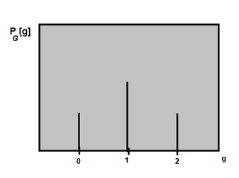 binary symmetric channelOk this is a trickier problem, and what I really liked about this one was that it is has such a great connection with electrical engineering. 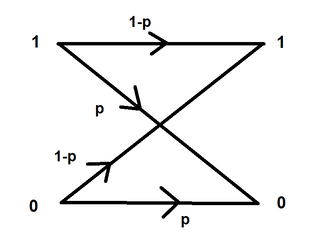 So, we are sending a 1000 bits into some data channel, and the probability there is a bit error (the bit was the wrong bit received, for example 1 is a 0 or 0 is a 1) = P[error] = 0.02. So 1-P[error] = success. So the question is, what is the probability there are 10 errors? Ok so first, we need to think about how many possible combinations are there if there are 10 errors out of 1000 bits sent into the channel. In order to figure out the total number of possibilities we do 1000 choose 10 (the combinations formula). We would then use the binomial distribution (since there are only 2 possible values, 1 or 0 to find the PMF: 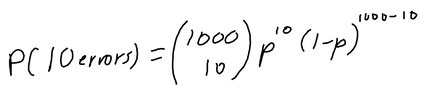 If we plug in P for 0.02, we get about P[10 errors] ~~ 0.0055, which is a relatively low probability!
0 Comments
I remember those fun middle school days when my math teacher used to teach us probability by bringing in a bunch of marbles and bags to find out what is the chance you pick a blue or red or pink marble, etc. Of course, we as college/high school students are gonna learn more than that. Probability is basically the 'science' and 'math' behind the uncertainty or certainty of an event. And it is applied EVERYWHERE. defining your sample spaceWhenever you are dealing with probability problems, you always need to define your sample space. The sample space is essentially the 'space' where you describe all of the possible outcomes of the event. It is also known as the symbol omega.  find the probability lawThe next step is to find your probability law. The probability law is basically the 'formula' used to assign probabilities to events of an experiment. For example, in some experiments (which we will talk about soon), the probabilities are determined by the area the events take up in the sample space. This is called a continuous probability model. In other cases, the probabilities of an event are determined by simple counting. For example, lets say this was your sample space: 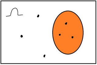 The orange part in the diagram is called an event. An event is just a collection of outcomes in a sample space. Lets say omega (sample space) consists of 6 equally likely elements. What is the probability you randomly choose a dot in the orange part of the board? Well, we know there are 6 different possible outcomes, because there are 6 different points. So, we basically divide the probability of the event with the total number of possible outcomes. In that case, the probability will be 3/6. So a half. Not that tricky, right? discrete uniform lawSo the example we just went over supports the discrete uniform law. The discrete uniform law says that if the sample space consists of n equally likely elements, and A, which is a subset of the sample space, consists of k elements, Probability of A = P(A) = k * 1/n = k/n Since all of the elements are equally likely to be chosen, each element has a probability of 1/n. Since A has k elements, the probability of A being chosen is k * 1/n = k/n. intro to axiomsOk, so far, so good. But what if the probability of something is negative? Is that even possible? How do we put rules and limits to these probability values? This is where axioms come in. Axioms are certain properties that probabilities need to follow in order to be valid. These are the three main probability axioms:
The first axiom is the non-negativity axiom. This axiom tells us that all probabilities have to be greater than or equal to 0. They CANNOT be negative. A probability of 0 indicates it is uncertain to happen, whereas a probability of 1 tells us that it is certain. The next axiom tells us that the probability of the sample space, or omega is 1. This makes sense because the sample space consists of all the possible outcomes. So it is absolutely certain of the event is going to happen, since it is in the sample space. The last axiom is famously known as the additivity axiom. The additivity axiom tells us that if there are two events that are disjoint (we will talk about this soon), then the probability of both the events together is the sum of the individual properties. I know that was a lot of info, so lets break it down: 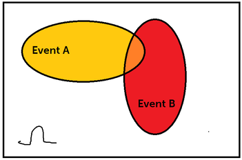 Look at the above diagram. Lets say we have two events in our sample space, Event A (highlighted in yellow), and Event B (highlighted in red). The intersection of these two events is the orange part. You denote the intersection of two events like this: A ∩ B. The intersection of two events means that there is a chance A and B can happen at the SAME TIME. The union of two events means there is a chance A or B can happen. You denote the union of two events like this: A ∪ B. So in the above example these two events were NOT disjoint. Disjoint events are two events or more where no intersection occurs. When both the events don't have an intersection they are disjoint. So, 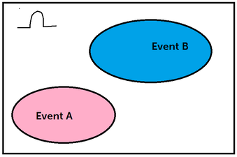 In this case, Events A and B are disjoint. So, back to the additivity axiom. The additivity axiom says that, if the intersection of two events is 0 (disjoint), then the P(A ∪ B) = P(A) + P(B). So this is saying that the union of these two events is the sum of the individual probabilities. Which makes sense because they are both separate events and we want to find whats the probability we land in event A or B.
Anyway, probability is a tricky but really cool concept to learn. Good luck! I never actually really understood the significance of eigenvalues and how it's applied visually until my Diff Equations class was over, which is not the best time to figure it out, but at least it'll help me for my future classes, lol. And, its actually pretty cool too!! Honestly, I think the time when I got super interested in learning about why these eigenvalues existed was when this scene came up in the Avengers Endgame.  When Tony Stark mentioned the word "eigenvalue" I was like, "OMG, OMG I actually kinda know this...kinda...that word is very familiar to me so it counts." LOL, yup, this is when I was like hmm I have to actually understand an eigenvalue's significance and application. So wow, that happened and I never would have expected an Avengers movie to squeeze in a quick lesson in Diff Equations and Linear Algebra. Anyways, getting back to the point, what is an eigenvalue? And what are these used for? For example, when you solve for an IVP (initial value problem) with matrices, you solve for the eigenvalues first by finding the determinant, and then you solve for the corresponding eigenvectors (from the eigenvalues), and then plug in the initial value equation to the general solution to find the value of the constants. That sounds terrible, but it's actually not too bad. It's basically just solving for linear equations except in a matrix you have to find the determinant. That's one way of using eigenvalues. But what are they? and what's their real world application? Eigenvalues and their corresponding eigenvectors summarize matrix data. Eigenvectors are vectors whose direction is not changed when some linear transformation is applied to the vector. For instance, 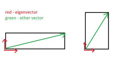 The red vector is an eigenvector since it never changes, even after a linear transformation has been applied. These vectors define the matrix of the transformation (scaling). For any matrix A (n x n square matrix), x, (a n x 1 vector) is an eigenvector of this matrix if the product of Ax is proportional to the product of x * eigenvalue. 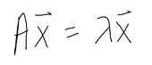 where x is the eigenvector, A is the matrix, and the lambda is the eigenvalue. When you solve for lambda using this formula, you will end up with: 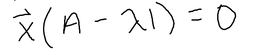 For this to be equal to 0, A has to equal lamda times I, where I is an identity matrix with the same dimensions as a, and lamda (eigenvalue) is just a scale factor. However, we are assuming that x is not a null vector, which means to satisfy the equation, A - lambda * I can't have an inverse. A matrix that is non-invertible has a determinant of 0. Therefore, we can conclude that, 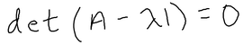 And we just use this equation to solve for eigenvalues of any n x n matrix.
Eigenvalues and eigenvectors of a certain matrix have tons of real world applications such as image compression, clustering in data science, predictions and page rank algorithms. |
Archives
May 2021
Topics
All
|
 RSS Feed
