|
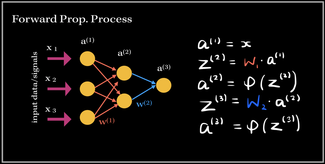
I've always wondered as to what happens in the 'backend' of the training process in Neural Networks. The training process is essentially the 'meat' of the model; without efficient and effective training the model will not be able to accurately predict/classify or accomplish a task with newly unseen data. Neural Networks have always been held as a very useful system in prediction analysis, recommendation engines, modeling and a lot more; it is because has the ability to extract complex patterns and relationships between the input and output data. This is because of the numerous layers of neural networks, that make the machine learning 'deep'. So what does the training process of this neurological-biological computer model-system (aka neural network) look like? It consists of two phases: 1). Forward Propagation and 2). Back propagation. Once we have preprocessed the dataset (such as normalization, reshaping your data to a specific dimension..etc.), we are ready for the training process. We first forward propagate our data—meaning we feed in the inputs into our built neural network. 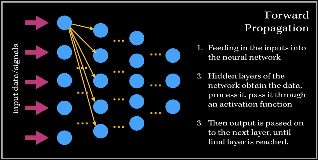 I like to think of forward propagation consisting of three simple steps: 1) Send in a data point (or a subset of training data points), 2) the layers obtain the data, process it (by computing the dot product), and pass it into some non-linear activation function (ReLU, Sigmoid, Leaky ReLU), 3). Output from previous layer is passed to next layer. The process continues until we have reached the final layer. Before we get into the deep math, let's define some variables. These definitions are applied to every example in this blog post!
 SO, what happens after we have passed an instance of our training dataset to the network? Back PropagationThis is where back propagation comes in. Back-propagation is essentially an algorithm used in training neural networks and is used to improve the model's performance/accuracy. Our neural network will update its parameters (weights and biases) once every time a number of samples is passed into the network (aka: an epoch in gradient descent algorithm). Basically, in Back Propagation, we need to adjust the weight parameters based on our loss function — whether it be calculating the mean squared loss, absolute mean loss or any other loss function we use — and our updated weights must head towards the right direction (in reducing the loss). Let's look at an example, and focus on one specific output neuron in a neural network model. We first pass in our input training data, and get a single output neuron of 0.5. However, the specific target value for the neuron is 1.0, so the cost function computes the error, and our optimizer uses the loss to back-propagate and change the weights to minimize the loss. This is why the process is at times called back-propagation of errors, since updates to one layer impact the next layer, and because of this backwards calculation technique, we are preventing redundant calculations. 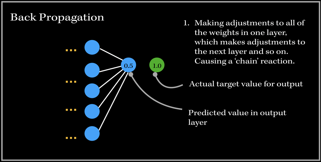 To do this, we need to figure out how much of an impact does a certain weight (between a node from one layer and a node from the previous layer) have on the cost function. Does the weight have a very low impact (ie. the cost function doesn't drastically differentiate when the weight parameter changes), or does it have a very important contribution towards minimizing the loss? In order to find this out, we need to look into a very important operation: partial derivatives. The Process
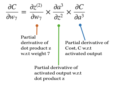
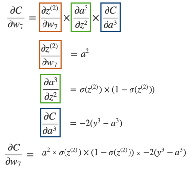
Let's go do a back propagation run through with an example. Say we had a neural network with 3 input neurons, 2 neurons in the hidden layer, and 1 output neuron. 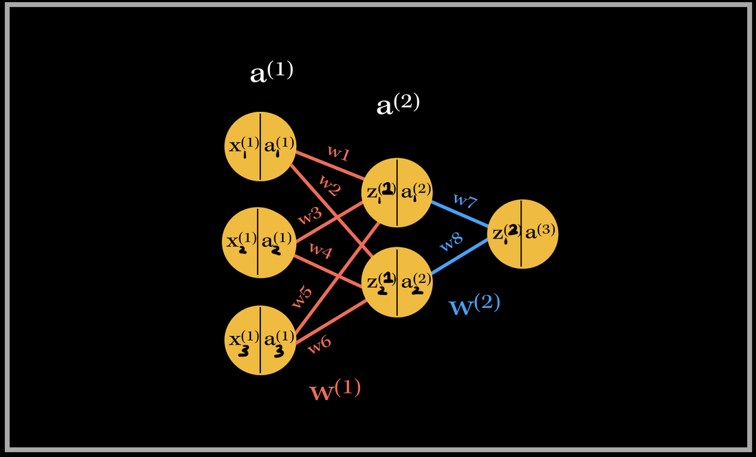 Neural Network Model with denoted weights, activation values, and dot product values (in neurons) NOTE: In each neuron, the number on the left side is the input, and number on the right side is the activated input (passed through activation sigmoid). Back-propagation of the output layerThe total number of weights in this network is 8. We have 6 weights in the first layer and 2 weights in the second layer. Let's first focus on the computing the partial derivative of the cost with respect to one of the weights contributing towards the output neuron: w7. What is the partial derivative of C, the cost, w.r.t to w7, weight 7?
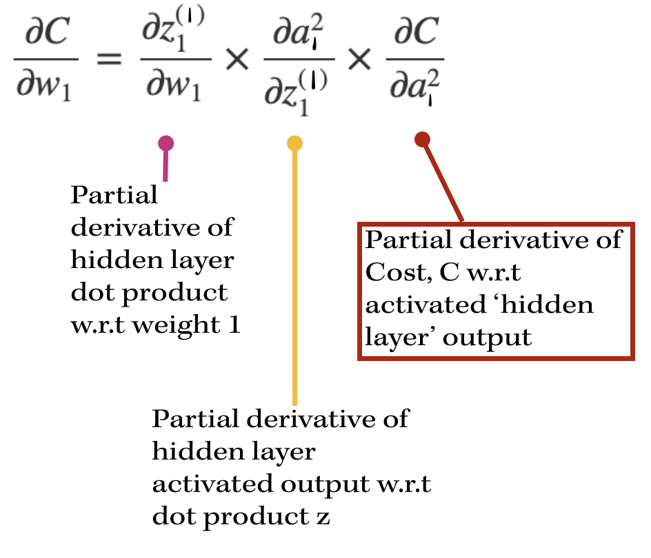
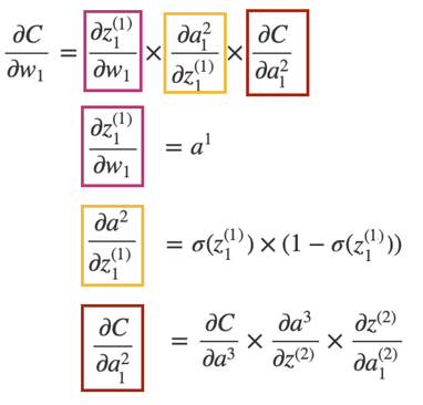
Back-propagation of a hidden layerNow, let's back propagate to the first layer, and compute the gradient of weight 1, w1. The partial derivatives will look slightly different this time, since the cost isn't directly associated with the hidden layer outputs. With our focus on weight 1, the partial derivative of the cost w.r.t w1 is going to depend on the partial derivative of the cost w.r.t. the output of the hidden layer neuron. This will look like:
So in order to find the partial derivative with respect to the hidden layer output, we need to include the next layer's weight's contribution towards the cost. Therefore, we need to include the weights that are being multiplied by the activation output of the particular hidden layer's neuron. In this case, it's only one weight: w7. However, if there are multiple weights contributing, we would have to add them to the equation as well.
The partial derivative of the Cost w.r.t. the hidden layer activation is broken down again into three parts: 1). First starting from the cost w.r.t to the output activation, then 2). the activation w.r.t the output dot product, 3). then the output dot product w.r.t. hidden layer activation. As you can see there are many terms being repeated in finding the updates for both weights 1 and 7!! This basically sums up finding the gradient of the network. As you can see, it requires lots of computation and derivatives!! Imagine the workload of computing the gradient vector of bigger neural networks with millions of parameters and neurons--backward propagation does this by using the previous layer's computations to compute the updates for the next layers! It's an amazing feat! Back propagating in action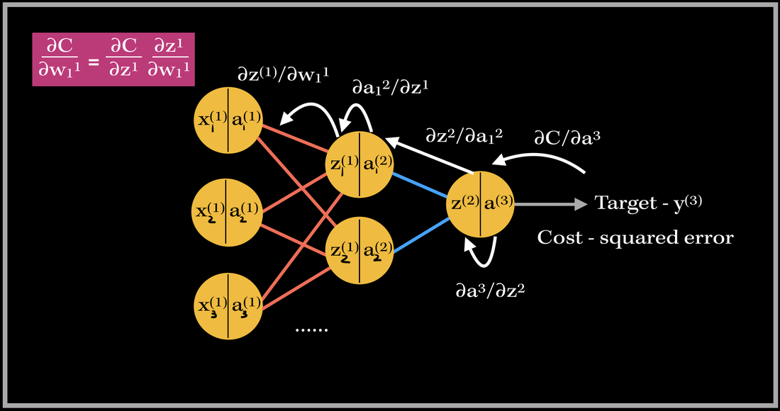 Back propagation in action for weight 1. So this is where 'back propagating the errors' comes into play. The image above is an example of back propagation in action for weight 1. The previous partial derivatives are reflected in the update value for weight 1. The white arrows show the path of each derivative computation for weight 1's update.
This same process occurs for every weight in the network during back propagation. Back Prop is one of the most important parts in training supervised learning neural network models! :)
1 Comment
When it comes to machine learning and computers being able to learn and recognize patterns--similar to what our brains do, (which is why ML/AI fields are so related to the neuroscience!) we want to be able to increase the accuracy and efficiency of our prediction algorithm. This is so that the prediction gets better and better, closer to the target value we are aiming towards achieving. Let's compare this situation to a more human-related real life scenario. Suppose you are studying for an exam. You have a set study plan, and followed the points in your plan to prepare. Unfortunately, you weren't too satisfied with your result, since your exam result was way off the targeted score you wanted to achieve. So, what do you do? Well, you would want to make some adjustments to your study plan in order to prepare for your next exam effectively and efficiently.  You would want to make adjustments based on what you think you should have worked on more, i.e. covering more broad topics next time, reading over applications, practicing more problems..etc. You are doing this because you learned from your past experience, and are making some changes to perform better, and get a better result. This is exactly what optimization in machine learning is all about. It's about making these small adjustments to see if an algorithm's accuracy is improving. The algorithm wants to get as close to the target value, and optimization techniques can allow us to choose and make adjustments to our paramaters of our machine learning model (also known as the weights), so the algorithm performs better next time. One of the most well known optimization methods used today is called the Stochastic Gradient Descent, (or SGD in short). How does this method work, and what certain adjustments does it make to our algorithm? Before we add the word "Stochastic"Before we dive into what Stochastic Gradient Descent is, lets take a look at what the term "Gradient Descent" means. When we want to increase the accuracy of a machine learning algorithm, we are looking for our error difference. What is the difference betweeen the target value and the predicted value from our model? 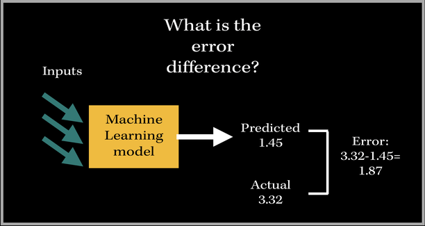 Let's say we had a model that outputs a numerical real valued number based on some arbitrary inputs. The predicted value (the value that is produced based on the model parameters) is 1.45. The actual target value is 3.32. This doesn't look that much of a good 'learning'-based model, since the target and predicted values aren't too close. The error difference is then 3.32-1.45 = 1.87. We want the target value to be close to the actual value, so how do we get a good understanding of whether the algorithm is functioning terribly or well? Cost FunctionWe can use a Cost Function to analyze the model's ability to understand and learn patterns and relationships between inputs and outputs. A cost function is usually a function of the error difference, and our goal in machine learning problems is to MINIMIZE the cost function. There are many cost functions we can use to optimize models. Examples are Mean Squared Error (MSE), Mean Absolute Error (MAE), and a lot of other more math-heavy trickier ones :) Now we might be thinking--why can't we just work with our error difference and minimize our error difference itself? Why do we have to work with a cost function? Our error function can also be negative--in this case it is 'minimized' in terms of the value, BUT, there still exists a huge difference between our predicted and actual values. So this is why we are going to instead focus on some function of our error, rather than just the error itself. For instance, if we are focusing on improving a single linear neuron's output prediction, (in a neural network), we will want to obtain a set of weights which will minimize the cost function. This means we will have to find the minima of the function--where is the lowest point of this particular function? This neuron has three inputs and 3 associated weights for each feature. The output is then the dot product of the weights and inputs, which is then passed into an activation function, such as ReLU. Now, how would we essentially train our model to adjust our weight parameters to improve the accuracy? Since we use functions to get to the output of this neuron, we need to do just the opposite to backpropagate, i.e. go back change the weight parameters to perform better. This means we are gonna get into derivatives. 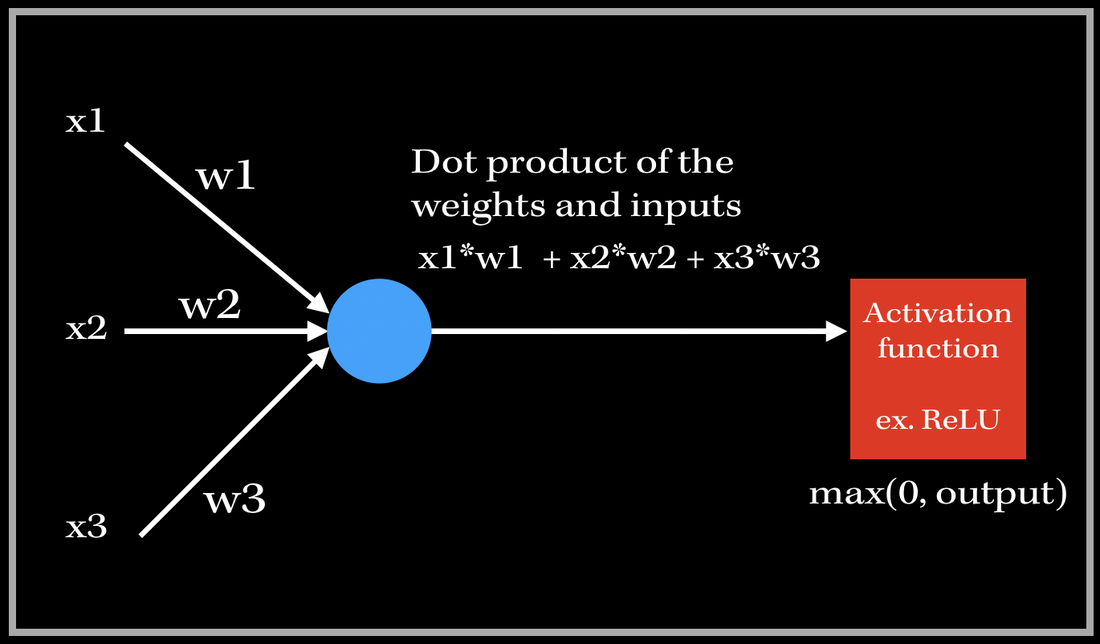 So we know that our cost function is technically a function of the weights, since computing the difference between the target and predicted value involves the predicted value, which involves the dot product of the weights and inputs. The main goal of gradient descent is to use the gradient to iteratively decrease the function of weights/cost function such that we find a set of weights for where the accuracy is maximized. The Gradient and the DescentWe can first set arbitrary values to our weights, for instance, starting from 0. Then, from that point, we need to find out which direction to go towards in order to reach the minimum value of the cost function. The gradient of the cost function tells us exactly that. The gradient, also denoted with a upside down triangle, represents the slope of the function with respect to each weight. The gradient of the cost function is basically a vector of partial derivatives with respect to each weight (ex. w1, w2,..etc). *Note: We are assumming this cost function is a strictly convex function, i.e. a function which has no more than 1 minimum point.* 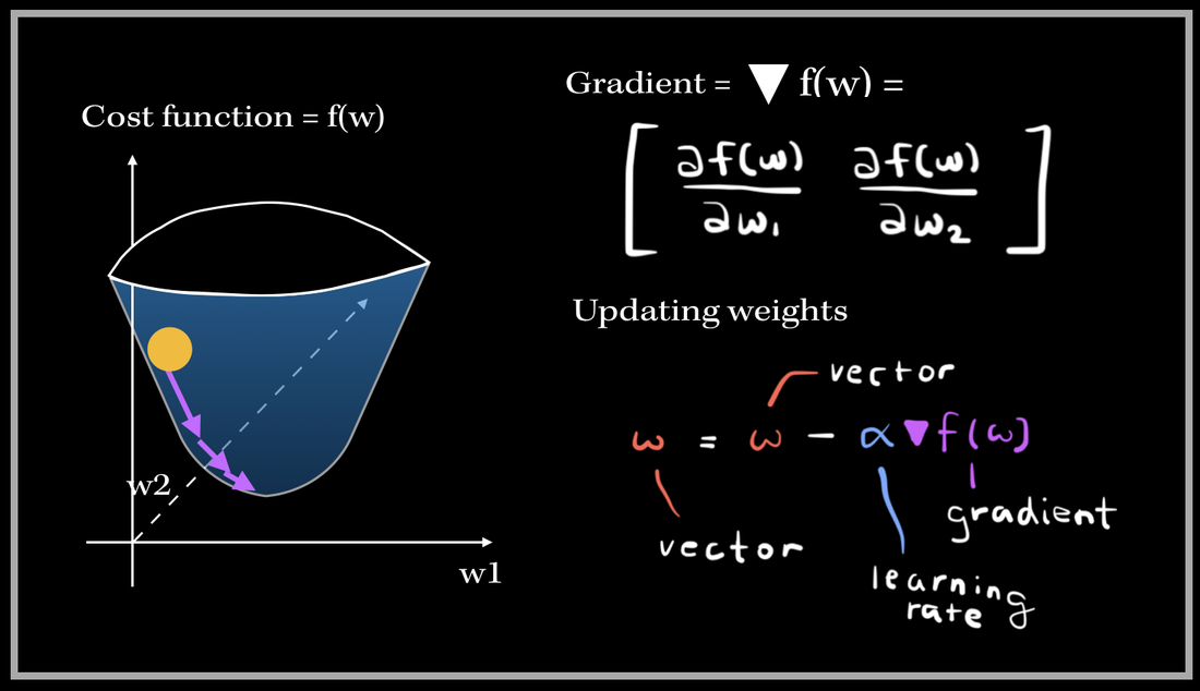 When we are updating our weights, we subtract the gradient multiplied by the step size with the old set of weights. The w in the equation above is basically a vector of weights, in this case a vector of two weights w1, w2. The gradient is also a vector with the partial derivatives with respect to w1, w2. This process of updating the weights iteratively happens until the gradient is at or at most close to 0 (this will indicate it's at a minima). The step size basically tells us how fast is the iterative process towards convergence. For instance, a small step size will slow down the convergence process, and a large step size might lead to an infinite amount of iterations..,divergence, which is not good! That is why it is so important to find the right step size amount. Back to the 'Stochastic'Ok, so know we looked into Gradient Descent, what does the term "Stochastic" mean? Stochastic is all about randomness. What can we do to this algorithm that involves randomness though? Though the Gradient Descent algorithm is very effective, it isn't too efficient for huge amounts of data and parameters. The Gradient Descent algorithm updates weights only after one epoch (complete pass of the training data). It would have to compute the gradient after every iteration (after one pass of all the training samples). With a large amount of features and weights, this can be computationally exhaustive, and time consuming. The Stochastic Gradient Descent, or SGD introduces a sense of randomness into this algorithm, which can make the process faster and more efficient. The dataset is shuffled (to randomize the process) and SGD essentially chooses one random data point at every iteration to compute the gradient. So instead of going through millions of examples, SGD using one random data point to update the parameters. This computationally makes the algorithm a bit more efficient. Consequently, it can lead to excessive 'noise' on the pathway to finding the minimum. For example: 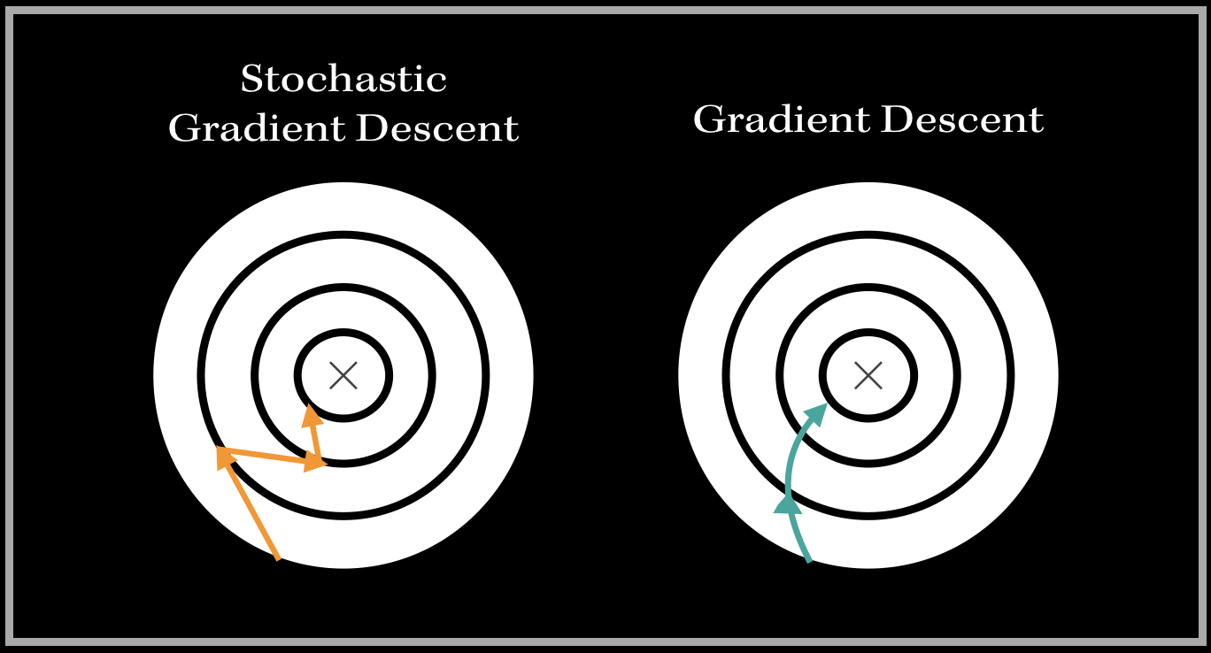 The Circle Maps represent the cost function, from the top-eye perspective or point of view. The path to finding the minimum point of the loss function looks very different for Gradient Descent and SGD. The trajectory towards the minimum looks very different for both of these variants of Gradient Descent. For SGD, the path is heading towards the minimum with harsh, and abrupt turns (because we are using random samples to update weights), and the path for the Gradient Descent algorithm is more smooth, and direct since we are using all of the training samples to compute the gradient. This is a very interesting aspect that looks visually different for both the optimizers. ApplicationsThe Stochastic Gradient Descent algorithm is one of the most used optimization algorithms in Machine Learning. It is very popular in deep learning and neural networks as well!
The Gradient Descent Algorithm has applications in Adaptive Filtering (learning based systems), and is used to optimize the filter's weights to minimize a cost value. An example of a particular Adaptive Filter is Noise Cancellation algorithm in headsets!!! :) |
Archives
December 2020
Topics
All
|
 RSS Feed
